Example scripts
A basic fitting script
The below script uses Gaussian descriptors with a neural network backend — the Behler-Parrinello approach — to train energies only to a training set made by the script. Note that most of the code is just generating the training data, and the training takes place in a couple of lines.
"""Simple test of the Amp calculator, using Gaussian descriptors and neural
network model. Randomly generates data with the EMT potential in MD
simulations."""

import os
from ase import Atoms, Atom, units
import ase.io
from ase.calculators.emt import EMT
from ase.build import fcc110
from ase.md.velocitydistribution import MaxwellBoltzmannDistribution
from ase.md import VelocityVerlet
from ase.constraints import FixAtoms

from amp import Amp
from amp.descriptor.gaussian import Gaussian
from amp.model.neuralnetwork import NeuralNetwork


def generate_data(count, filename='training.traj'):
    """Generates test or training data with a simple MD simulation."""
    if os.path.exists(filename):
        return
    traj = ase.io.Trajectory(filename, 'w')
    atoms = fcc110('Pt', (2, 2, 2), vacuum=7.)
    atoms.extend(Atoms([Atom('Cu', atoms[7].position + (0., 0., 2.5)),
                        Atom('Cu', atoms[7].position + (0., 0., 5.))]))
    atoms.set_constraint(FixAtoms(indices=[0, 2]))
    atoms.calc = EMT()
    atoms.get_potential_energy()
    traj.write(atoms)
    MaxwellBoltzmannDistribution(atoms, 300. * units.kB)
    dyn = VelocityVerlet(atoms, dt=1. * units.fs)
    for step in range(count - 1):
        dyn.run(50)
        traj.write(atoms)


generate_data(20)

calc = Amp(descriptor=Gaussian(),
           model=NeuralNetwork(hiddenlayers=(10, 10, 10)))
calc.train(images='training.traj')
Note you can monitor the progress of the training by typing amp-plotconvergence amp-log.txt, which will create a file called convergence.pdf.
A basic script with forces
The below script trains both energy and forces to the same training set as above. Note this may take some time to run, which will depend upon the initial guess for the neural network parameters that is randomly generated. Try decreasing the force_rmse convergence parameter if you would like faster results.
"""Simple test of the Amp calculator, using Gaussian descriptors and neural
network model. Randomly generates data with the EMT potential in MD
simulations."""

import os
from ase import Atoms, Atom, units
import ase.io
from ase.calculators.emt import EMT
from ase.build import fcc110
from ase.md.velocitydistribution import MaxwellBoltzmannDistribution
from ase.md import VelocityVerlet
from ase.constraints import FixAtoms

from amp import Amp
from amp.descriptor.gaussian import Gaussian
from amp.model.neuralnetwork import NeuralNetwork
from amp.model import LossFunction


def generate_data(count, filename='training.traj'):
    """Generates test or training data with a simple MD simulation."""
    if os.path.exists(filename):
        return
    traj = ase.io.Trajectory(filename, 'w')
    atoms = fcc110('Pt', (2, 2, 2), vacuum=7.)
    atoms.extend(Atoms([Atom('Cu', atoms[7].position + (0., 0., 2.5)),
                        Atom('Cu', atoms[7].position + (0., 0., 5.))]))
    atoms.set_constraint(FixAtoms(indices=[0, 2]))
    atoms.calc = EMT()
    atoms.get_potential_energy()
    traj.write(atoms)
    MaxwellBoltzmannDistribution(atoms, 300. * units.kB)
    dyn = VelocityVerlet(atoms, dt=1. * units.fs)
    for step in range(count - 1):
        dyn.run(50)
        traj.write(atoms)


generate_data(20)

calc = Amp(descriptor=Gaussian(),
           model=NeuralNetwork(hiddenlayers=(10, 10, 10)))
calc.model.lossfunction = LossFunction(convergence={'energy_rmse': 0.02,
                                                    'force_rmse': 0.02})
calc.train(images='training.traj')
Note you can monitor the progress of the training by typing amp-plotconvergence amp-log.txt, which will create a file called convergence.pdf.
Examining fingerprints
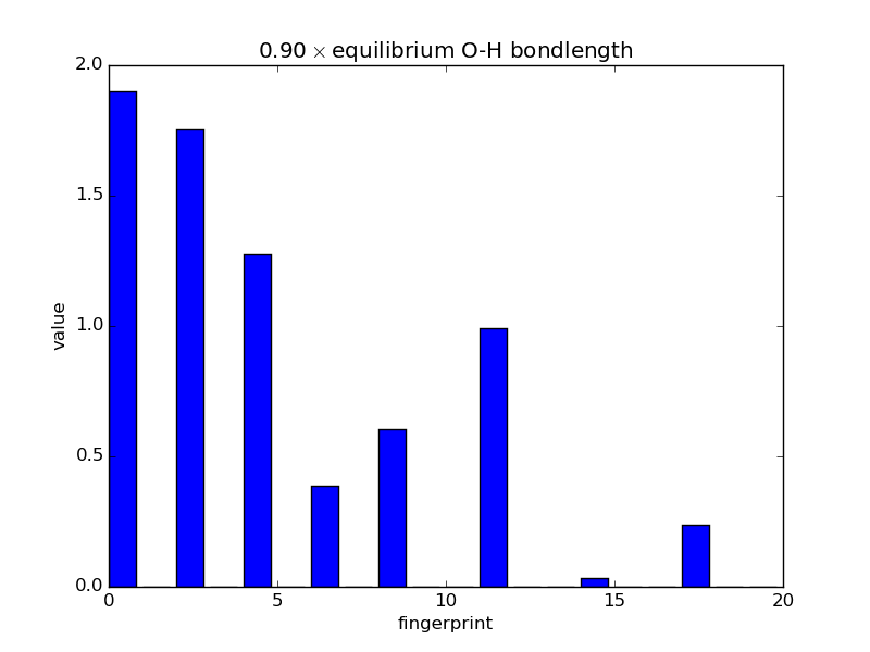
With the modular nature, it’s straightforward to analyze how fingerprints change with changes in images. The below script makes an animated GIF that shows how a fingerprint about the O atom in water changes as one of the O-H bonds is stretched. Note that most of the lines of code below are either making the atoms or making the figure; very little effort is needed to produce the fingerprints themselves—this is done in three lines.
# Make a series of images.
import numpy as np
from ase.structure import molecule
from ase import Atoms
atoms = molecule('H2O')
atoms.rotate('y', -np.pi/2.)
atoms.set_pbc(False)
displacements = np.linspace(0.9, 8.0, 20)
vec = atoms[2].position - atoms[0].position
images = []
for displacement in displacements:
    atoms = Atoms(atoms)
    atoms[2].position = (atoms[0].position + vec * displacement)
    images.append(atoms)

# Fingerprint using Amp.
from amp.descriptor.gaussian import Gaussian
descriptor = Gaussian()
from amp.utilities import hash_images
images = hash_images(images, ordered=True)
descriptor.calculate_fingerprints(images)

# Plot the data.
from matplotlib import pyplot

def barplot(hash, name, title):
    """Makes a barplot of the fingerprint about the O atom."""
    fp = descriptor.fingerprints[hash][0]
    fig, ax = pyplot.subplots()
    ax.bar(range(len(fp[1])), fp[1])
    ax.set_title(title)
    ax.set_ylim(0., 2.)
    ax.set_xlabel('fingerprint')
    ax.set_ylabel('value')
    fig.savefig(name)

for index, hash in enumerate(images.keys()):
    barplot(hash, 'bplot-%02i.png' % index,
            '%.2f$\\times$ equilibrium O-H bondlength'
            % displacements[index])

# For fun, make an animated gif.
import os
filenames = ['bplot-%02i.png' % index for index in range(len(images))]
command = ('convert -delay 100 %s -loop 0 animation.gif' %
           ' '.join(filenames))
os.system(command)