Theory

According to Born-Oppenheimer approximation, the potential energy of an atomic configuration can be assumed as a function of only nuclei positions. Potential energy is in general a very complicated function that in theory can be found by directly solving the Schrodinger equation. However, in practice, exact analytical solution to the many-body Schrodinger equation is very difficult (if not impossible). Taking into account this fact, the idea is then to approximate the potential energy with a regression model:

\[\textbf{R}\xrightarrow{\text{regression}}E=E(\textbf{R}),\]

where \(\textbf{R}\) is the position of atoms in the system.

Atomic representation of potential energy

In order to have a potential function which is simultaneously applicable to systems of different sizes, the total potential energy of the system can to be broken up into atomic energy contributions:

\[E(\textbf{R})=\sum_{\text{atom}=1}^{N}E_\text{atom}(\textbf{R}).\]

The above expansion can be justified by assembling the atomic configuration by bringing atoms close to each other one by one. Then the atomic energy contributions can be approximated using a regression method:

\[\textbf{R}\xrightarrow{\text{regression}}E_\text{atom}=E_\text{atom}\left(\textbf{R}\right).\]

Descriptor

A better interpolation can be achieved if an appropriate symmetry function \(\textbf{G}\) of atomic coordinates, approximating the functional dependence of local energetics, is used as the input of regression operator:

\[\textbf{R}\xrightarrow{\textbf{G}}\textbf{G}\left(\textbf{R}\right)\xrightarrow{\text{regression}}E_\text{atom}=E_\text{atom}\left(\textbf{G}\left(\textbf{R}\right)\right).\]

Gaussian

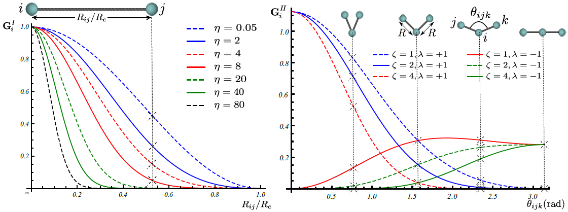
Gaussian descriptor \(\textbf{G}\) as a function of pair-atom distances and three-atom angles, has been suggested by Behler [1], and is implemented within Amp. Radial fingerprint of Gaussian type captures interaction of atom \(i\) with all atoms \(j\) as the sum of Gaussians with width \(\eta\) and center \(R_s\),

\[\begin{split}G_{i}^{I}=\sum^{\tiny{\begin{array}{c} \text{atoms j within }R_c\\ \text{ distance of atom i} \end{array}}}_{j\ne i}{e^{-\eta(R_{ij}-R_s)^2/R_c^2}f_c\left(R_{ij}\right)}.\end{split}\]

The next type is the angular fingerprint accounting for three-atom interactions. Gaussian angular fingerprint is computed for all triplets of atoms \(i\), \(j\), and \(k\) by summing over the cosine values of the angles \(\theta_{ijk}=\cos^{-1}\left(\displaystyle\frac{\textbf{R}_{ij}.\textbf{R}_{ik}}{R_{ij}R_{ik}}\right)\), (\(\textbf{R}_{ij}=\textbf{R}_{i}-\textbf{R}_{j}\)), centered at atom \(i\), according to

\[\begin{split}G_{i}^{II}=2^{1-\zeta}\sum^{\tiny{\begin{array}{c} \text{atoms j, k within }R_c\\ \text{ distance of atom i} \end{array}}}_{\scriptsize\begin{array}{c} j,\,k\ne i \\ (j\ne k) \end{array}}{\left(1+\lambda \cos \theta_{ijk}\right)^\zeta e^{-\eta\left(R_{ij}^2+R_{ik}^2+R_{jk}^2\right)/R_c^2}f_c\left(R_{ij}\right)f_c\left(R_{ik}\right)f_c\left(R_{jk}\right)},\end{split}\]

with parameters \(\lambda\), \(\eta\), and \(\zeta\). The function \(f_c\left(R_{ij}\right)\) in the above equations is the cutoff function defining the energetically relevant local environment with value one at \(R_{ij}=0\) and zero at \(R_{ij}=R_{c}\), where \(R_c\) is the cutoff radius. In order to have a continuous force-field, the cutoff function \(f_c\left(R_{ij}\right)\) as well as its first derivative should be continuous in \(R_{ij}\in\left[0,\infty\right)\). One possible expression for such a function as proposed by Behler [1] is

\[\begin{split}f_{c}\left(R_{ij}\right)== \begin{cases} &0.5\left(1+\cos\left(\pi\displaystyle\frac{R_{ij}}{R_c}\right)\right)\qquad \text{for}\;\: R_{ij}\leq R_{c},\\ &0\qquad\qquad\qquad\qquad\quad\quad\quad\:\: \text{for}\;\: R_{ij}> R_{c}.\\ \end{cases}\end{split}\]

Figure below shows how components of fingerprints \(\textbf{G}_{i}^{I}\) and \(\textbf{G}_{i}^{II}\) change with, respectively, distance \(R_{ij}\) between pair atoms \(i\) and \(j\) and valence angle \(\theta_{ijk}\) between triplet of atoms \(i\), \(j\), and \(k\) with central atom \(i\):

Zernike

Three-dimensional Zernike descriptor is also available inside Amp, and can be used as the atomic environment descriptor. Zernike-type descriptor has been previously used in the machine-learning community extensively, but it has been suggested here as the first time for representing chemical local environment. Zernike moments are basically a tensor product between spherical harmonics complete and orthogonal on the surface of unit sphere, and Zernike polynomials complete and orthogonal within the unit sphere. Zernike descriptor components for each integer degree are then defined as the norm of Zernike moments with the same corresponding degree. For more details on the Zernike descriptor the reader is referred to the nice paper of Novotni and Klein [2].

Inspired by Bartok et. al. [3], to represent the local chemical environment of atom \(i\), an atomic density function \(\rho_{i}(\mathbf{r})\) is defined for each atomic local environment as the sum of delta distributions shifted to atomic positions:

\[\begin{split}\rho_{i}(\mathbf{r}) = \sum_{j\neq i}^{\tiny{\begin{array}{c} \text{atoms j within }R_c\\ \text{ distance of atom i} \end{array}}}\eta_{j}\delta\left(\mathbf{r}-\mathbf{R}_{ij}\right)f_{c}\left(\|\mathbf{R}_{ij}\|\right),\end{split}\]

Next components of Zernike descriptor are computed from Zernike moments of the above atomic density destribution for each atom \(i\).

Figure below show how components of Zernike descriptor vary with pair-atom distance, three-atom angle, and four-atom dehidral angle. It is important to note that components of the Gaussian descriptor discussed above are non-sensitive to the four-atom dehidral angle of the following figure.

Bispectrum

Bispectrum of four-dimensional spherical harmonics have been suggested by Bartok et al. [3] to be invariant under rotation of local atomic environment. In this approach, the atomic density distribution defined above is first mapped onto the surface of unit sphere in four dimensions. Consequently, Bartok et al. have shown that the bispectrum of this mapping can be used as atomic environment descriptor. We refer the reader to the original paper [3] for mathematical details. Worth to mention that this approach of describing local environment is also available inside Amp.

Regression Model

The general purpose of the regression model \(x\xrightarrow{\text{regression}}y\) with input \(x\) and output \(y\) is to approximate the function \(y=f(x)\) by using sample train data points \((x_i, y_i)\). The intent is to later use the approximated \(f\) for input data \(x_j\) (other than \(x_i\) in the train data set), and make predictions for \(y_j\). Typical regression models include, but are not limited to, Gaussian processes, support vector regression, and neural network.

Neural network model

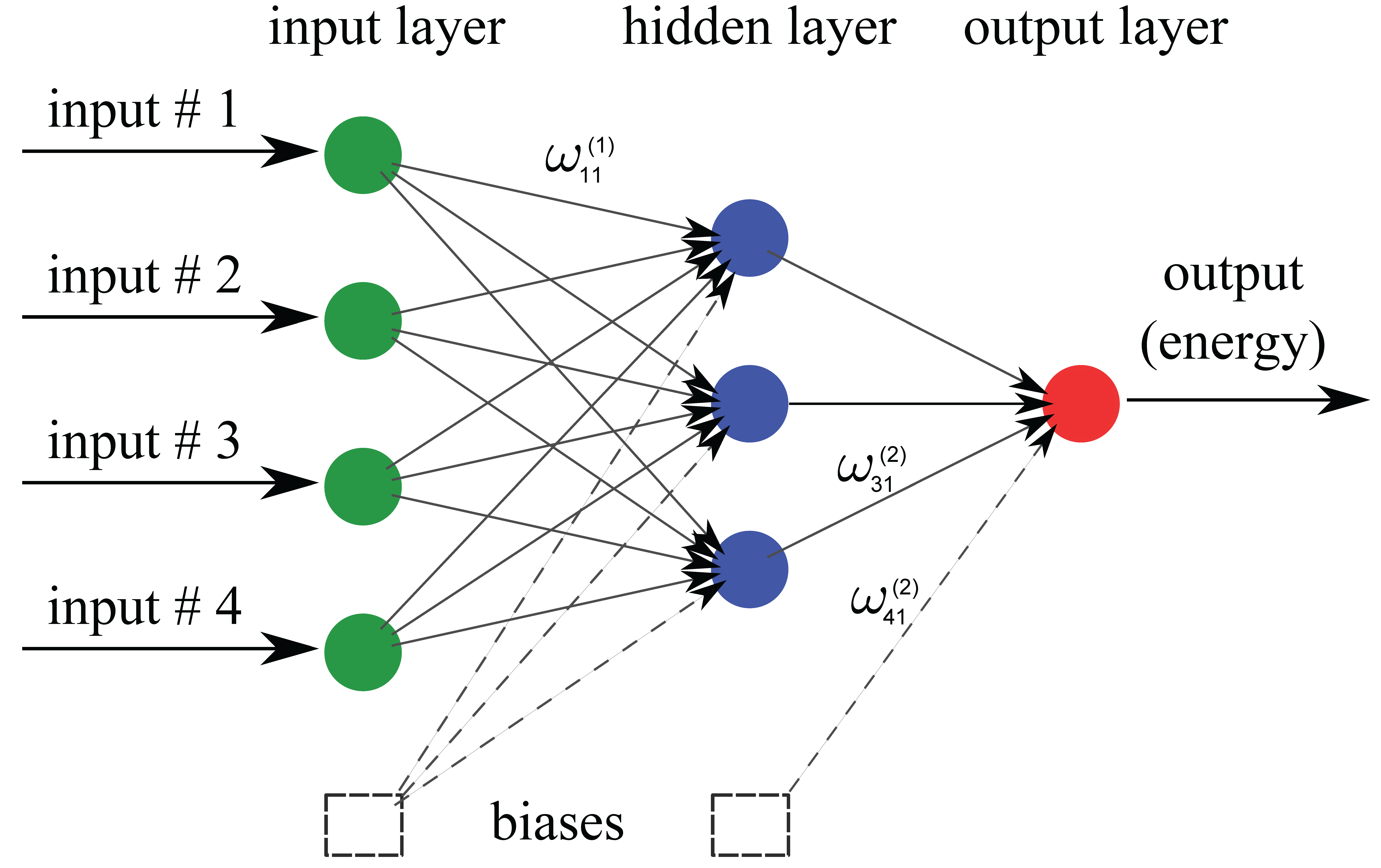
Neural network is basically a very simple model of how the nervous system processes information. The first mathematical model was developed in 1943 by McCulloch and Pitts [4] for classification purposes; biological neurons either send or do not send a signal to the neighboring neuron. The model was soon extended to do linear and nonlinear regression, by replacing the binary activation function with a continuous function. The basic functional unit of a neural network is called “node”. A number of parallel nodes constitute a layer. A feed-forward neural network consists of at least an input layer plus an output layer. When approximating the PES, the output layer has just one neuron representing the potential energy. For a more robust interpolation, a number of “hidden layers” may exist in the neural network as well; the word “hidden” refers to the fact that these layers have no physical meaning. A schematic of a typical feed-forward neural network is shown below. In each node a number of inputs is multiplied by the corresponding weights and summed up with a constant bias. An activation function then acts upon the summation and an output is generated. The output is finally sent to the neighboring neuron in the next layer. Typically used activation functions are hyperbolic tangent, sigmoid, Gaussian, and linear function. The unbounded linear activation function is particularly useful in the last hidden layer to scale neural network outputs to the range of reference values. For our purpose, the output of neural network represents energy of atomic system.

References:

1. “Atom-centered symmetry functions for constructing high-dimensional neural network potentials”, J. Behler, J. Chem. Phys. 134(7), 074106 (2011)
2. “Shape retrieval using 3D Zernike descriptors”, M. Novotni and R. Klein, Computer-Aided Design 36(11), 1047–1062 (2004)
3. “Gaussian approximation potentials: The accuracy of quantum mechanics, without the electrons”, A.P. Bart’ok, M.C. Payne, R. Kondor and G. Csanyi, Physical Review Letters 104, 136403 (2010)
4. “A logical calculus of the ideas immanent in nervous activity”, W.S. McCulloch, and W.H. Pitts, Bull. Math. Biophys. 5, 115–133 (1943)